Estimating Building Operating Schedules

Introduction

When estimating the baseline consumption of a building, it is often necessary to estimate its operating schedule, i.e. the energy consumption observations that correspond to the building's HVAC systems operating in setpoint mode and the observations that correspond to the setback mode. The Meval tool uses the operating schedule so as to decide which data to use in order to fit its underlying physics-based model. The Time-of-Week-and-Temperature (TOWT) model requires schedule information so as to differentiate the coefficients that capture temperature effects in setpoint mode from the coefficients for the setback mode.

In this article, we explore the mathematical foundations of the method that Meval uses to estimate a building's operate schedule, and provide practical guidance for implementing this technique in your M&V projects.

Expectation-Maximization with Two Regression Models for Schedule Inference

In many buildings, observed energy consumption data can be regarded as the result of a mixture of hidden operating modes. In particular, energy consumption may follow one pattern when a building is unoccupied (setback mode) and another when it is occupied (setpoint mode). The challenge is that the operating state is not directly observed; we only observe outdoor air temperature and energy consumption. One way to address this problem is to apply the Expectation-Maximization (EM) algorithm with two regression models, each representing one hidden regime.

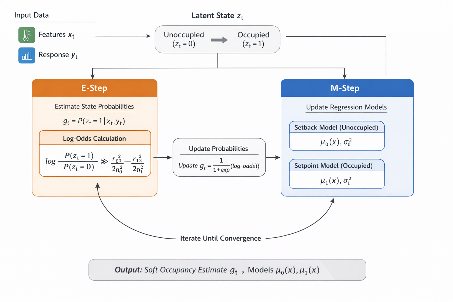
A formal way to describe the process that we assume generates the energy consumption data is:

y_t \mid z_t = k \sim \mathcal{N}(\mu_k(x_t), \sigma_k^2), \quad k \in \{0,1\}

Here, $y_t$ represents the observed energy consumption, $z_t$ is the hidden state (0 for setback and 1 for setpoint), $x_t$ is a time series of occupancy-independent inputs (mainly outdoor temperature) and $\mu_0(x_t), \mu_1(x_t)$ are the regression functions to be estimated. $\sigma_0, \sigma_1$ are the noise levels.

The EM algorithm alternates between estimating the hidden state probabilities (E-step) and updating the regression models (M-step).

E-Step: Estimating State Probabilities

Given the current regression models, the step computes how well each model explains each observation. This is reflected on each model's residuals:

r_{0,t} = y_t - \mu_0(x_t), \quad r_{1,t} = y_t - \mu_1(x_t)

We compare the likelihood of each state using a log-odds formulation:

logOdds = \log \frac{P(z_t = 1 \mid x_t, y_t)}{P(z_t = 0 \mid x_t, y_t)} = \frac{r_{0,t}^2}{2\sigma_0^2} - \frac{r_{1,t}^2}{2\sigma_1^2}

The log-odds are converted into a probability via the logistic function. This is the probability that the building is in setpoint mode at time t:

g_t = \frac{1}{1 + \exp(-logOdds)}

M-Step: Updating the Models

Using the current probabilities $g_t$ , we re-fit both regression models. The setback model is fit using a weighted regression with weights $w_{0,t} = (1 - g_t)^2$ . This forces the model to focus mainly on observations that are described better by it. The setpoint model is trained with weights $w_{1,t} = g_t^2$ .

Each component's noise level is updated from its weighted residuals (to ensure that each model is evaluated relative to its own uncertainty):

\sigma_k^2 = \frac{\sum_{t=1}^n w_{k,t}, r_{k,t}^2} {\sum_{t=1}^n w_{k,t}}

The E-step and M-step are repeated until convergence, typically when:

\frac{1}{n} \sum_{t=1}^n \left| g_t^{(i)} - g_t^{(i-1)} \right| < \varepsilon

The Expectation-Maximization algorithm as flowchart — The Expectation-Maximization algorithm

Practical considerations

When implementing this approach in your M&V projects, consider the following:

Ensure separability between the two regression models

A good way to achieve this is to make sure that the setpoint model is more flexible and has access to more features than the setback model.

Borrow statistical strength from recurrent patterns

When estimating $g_t$ , add a rule so that when it is highly uncertain (~0.5), pull the estimation toward confident values that are nearby in time.

Exploit features that correlate strongly with the hidden schedule without breaking EM

Such features should be kept out of the regression models. If you include them there, you collapse the distinction between the two regimes, which breaks the whole point of the algorithm. Instead, train a classifier that learns to map the values of the features to the schedule probabilities (rounded to 0 and 1, and using the actual probabilities as training weights). In this way, you will get a mixture of experts (in effect, each of the regression models is an expert) with a learned gating function that informs the algorithm which expert to trust.

Example

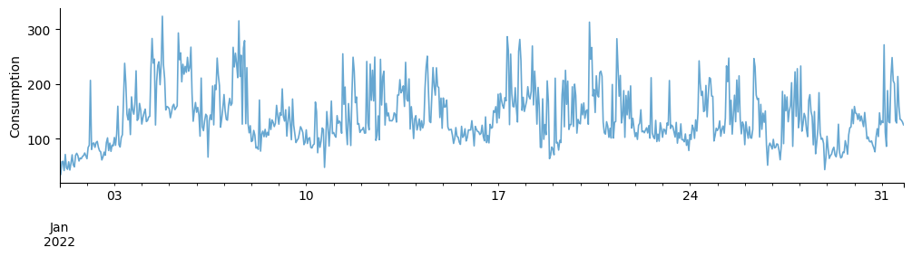
We can create a synthetic dataset with real temperature data, a binary schedule as ground truth, a setpoint (occupied) regime with stronger outdoor temperature sensitivity and a setback (unoccupied) regime with weaker response to temperature, and an autoregressive generator for the number of occupants that is linked to internal heat gains. The first month of the data is shown below (first month of the data):

The first month of the synthetic dataset

One way to view the schedule estimation process is as clustering the energy consumption around two different models. The synthetic dataset is rather easy to cluster, and the EM algorithm splits the data as shown below:

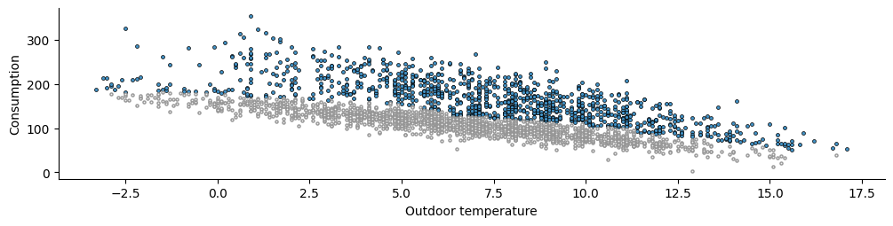
Since the dataset is not very hard to separate, we could have gotten similar results by fitting a global model of energy consumption as function of outdoor temperature and, then, assume that all observations above its prediction belong to the setpoint regime and all observations below to the setback regime.

However, EM allows us to do something that the previous heuristic cannot. Suppose you have a feature that you know it strongly correlates to the hidden schedule, but not necessarily to the energy consumption:

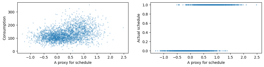
Adding this feature to your global predictive model will make the heuristic perform much worse (in this case binary classification accuracy drops from 0.90 to 0.67). The EM algorithm will improve its performance (accuracy goes from 0.91 to 0.93). All you need to do is fit a gating model during the E-step that nudges the schedule estimations towards the model's predictions.

Conclusion

Simple heuristics may work for buildings that follow very predictable schedules, but, in most cases, smart algorithms can help get the most insights from the available data. In this case, Expectation-Maximization is a powerful tool for estimating hidden states in the available data of a building. This method is already utilized by Meval to enable automated and statistically rigorous M&V calculations.