Introduction
All predictive models produce predictions that deviate from the observed target values. In fact, a perfect match between observed and predicted data implies that the model has learned noise in addition to the underlying signal. This condition is known as overfitting. Overfitted models have limited ability to predict accurately on data that they have not already seen. Accordingly, deviations should be expected. Part of the deviations can be attributed to the noise / stochasticity in the data, and part of it to the inability of the model to capture the real dynamics of the data due to unobserved features, unmodeled dynamics and misspecification of the model structure.
Close-form formulas for the uncertainty of energy savings include the number of observations as input. As an example, ASHRAE Guideline 14 prescribes that the Fractional Savings Uncertainty (FSU) is estimated as:
Where is the t-statistic for the desired confidence level, is the number of pre-retrofit data points, is the number of post-retrofit data points, is the coefficient of variation of the root mean square error of the baseline model, is the mean baseline energy consumption, and is the mean post-retrofit energy consumption.
So, what is the number of data points? Energy consumption is autocorrelated (past values influence the future ones). But to accurately estimate the savings uncertainty, we need independent observations. This means that if we have 100 data points, but we must take every fifth in order to break the autocorrelation, in effect we only have 20 data points. This is why ignoring autocorrelation leads to underestimated uncertainty intervals.
Although there are methods for accounting for autocorrelation in formulas that expect independent data points, this article presents an alternative method for estimating uncertainty: the conformal prediction approach.
Conformal Prediction
Conformal prediction is based on the idea that the errors of the model when applied on data that were not seen during training, can provide information about the uncertainty inverval around the model's predictions given a desired miscoverage level :
Here, is the prediction interval for the as a function of ( implies data that the model is applied on).
The main algorithm for the conformal prediction is simple:
Define score function
Compute quantile
Construct interval
This process has a drawback though: it produces uncertainty intervals of fixed width. However, our predictive model may be able to predict more accurately in some feature sub-spaces than others. To make the intervals adaptive, we can define a difficulty function that maps our features to the residuals' variance. A simple choice is to fit a model that maps our features to the . Then, the conformal score becomes:
We can now calculate the prediction sets using the rule:
Dealing with Autocorrelation
We haven't said anything yet about autocorrelation, but we should note that the method as presented so far cannot gracefully deal with it. However, there is a straightforward extension, called Block Conformal Prediction, that can.
Block conformal prediction corrects for autocorrelation by grouping consecutive residuals into blocks and calibrating the prediction intervals based on block-level conformity scores (the higher the score, the larger the error in that block). A common choice is the maximum absolute residual in the block. Block lengths should be long enough to smooth out the autocorrelation structure (a length of 24 hours is reasonable). This approach is similar to the way block bootstrap is used to sample blocks of residuals when the goal is to generate samples that respect the temporal dependence of the data.
The rest of the conformal prediction methodology remains the same. Difficulty models can still be used to normalize the scores, but the normalized scores are now grouped by blocks (blocks solve temporal dependency, while normalization deals with differences in variance). The quantiles for the intervals are calculated using block-level scores instead of individual observation-level ones.
The Link with Cross-Validation
Generating the conformal blocks can be done in a process of cross-validation. Cross-validating for M&V requires a balance between: (a) not penalizing a model by asking it to perform a task that is different than the M&V task, and (b) not making it easy for it to exploit autocorrelation and learn to trivially interpolate between values. The standard K-fold cross-validation is an example of the first case. A well-designed M&V model should drop any calendar features that represent months or weeks if the provided data do not span a full year (otherwise the model would have to extrapolate to missing months, which is always much worse than just ignoring month / week features altogether). As a result, K-fold cross-validation inflates the error for M&V models.
At the same time, randomly shuffling data points would allow predictive models (especially flexible, non-linear ones such as tree models, neural nets or models with nearest-neighbor-like behavior) to exploit autocorrelation (often called data leakage via autocorrelation) and, as a result, underestimate the out-of-sample error. Contrary to common perception, time-aware cross-validation is also not appropriate for M&V. Time-aware validation is appropriate for forecasting tasks but M&V is not forecasting; it is a comparison between similar outdoor conditions and indoor states before and after an event.
A better approach to cross-validation for M&V is to split data into weeks and randomly select those that will be used for training the model and those that will be used to test it. If calendar features are encoded as one-hot, stratified sampling should be used so that all months are present in the test sample. If calendar features are encoded as Fourier features, stratified sampling is not necessary.
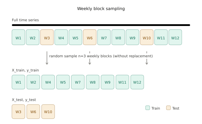
The residuals that are generated through a weekly block sampling can be used for calculating performance metrics such as the CVRMSE (Coefficient of Variation of the Root-Mean-Square Error) and NMBE (Normalized Mean Bias Error). But, they can also be used as a pool for calculating the conformal scores of the block conformal prediction method, since the conformal blocks (24-hour length) can be extracted from the test sample (168-hour blocks).
Example
We can evaluate uncertainty intervals based on coverage and average width. Coverage defines the probability that a calculated interval contains the true value of the labels. We can calculate the coverage at different confidence levels and, then, sum over the absolute values of the differences between each coverage value and the corresponding confidence level. The smaller the average of the differences, the better the intervals fit on the data. On the other hand, the wider the width of the intervals, the more conservative the uncertainty estimation.
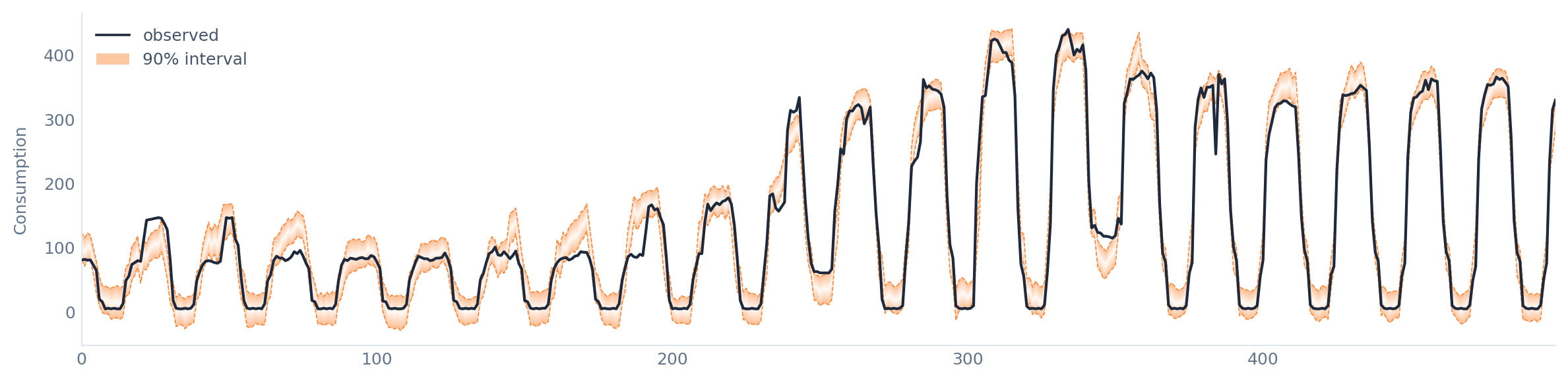
As an example, we can use the energy consumption for cooling of a real shopping mall. First, we adopt the false assumption of data independence. In this case, the average coverage difference is 0.10 and the average width for the 90% confidence level is 50.5 kWh.
To deal with autocorrelation, we can use block bootstrap, where instead of sampling individual residuals, we sample contiguous blocks. For this dataset, autocorrelation diminishes after 10 hours, so 10 hours will be the block length. The average coverage difference becomes 0.003 and the average width for the 90% confidence level is 44.2 kWh. So, dealing with autocorrelation significantly improved our uncertainty estimation.
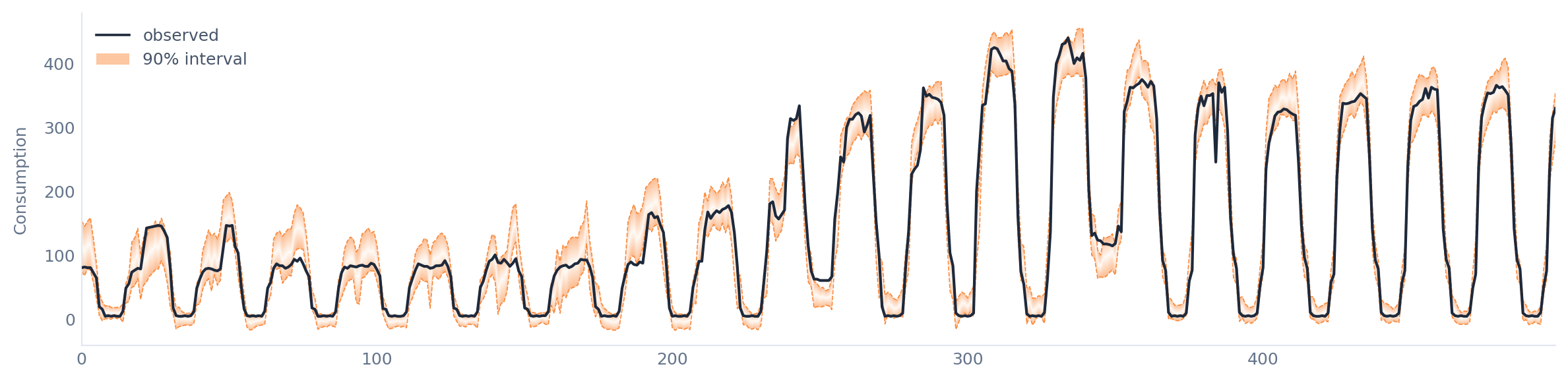
The method that Meval uses learns the residuals' scale so that to generate intervals of adaptive width. In this case, the average coverage difference is 0.01 and the average width for the 90% confidence level is 34 kWh. So, with a small sacrifice in coverage, we get much tighter uncertainty intervals, which translates in tigher intervals for the cumulative energy savings.
From Predictions to Cumulative Savings
The recipe that Meval uses to generate uncertainty intervals for cumulative savings estimations is:
Generate uncertainty intervals
Approximate residual distribution
Use a Gaussian copula sampler
Create trajectories of energy savings
Construct intervals
Conclusion
Modern machine learning methods offer a useful alternative to uncertainty estimation for M&V, often outperforming the methods that rely on distributional assumptions.